بحث مخصص من جوجل فى أوفيسنا

Custom Search
|


lionheart
-
Posts
671 -
تاريخ الانضمام
-
تاريخ اخر زياره
-
Days Won
28
نوع المحتوي
التقويم
المنتدى
مكتبة الموقع
معرض الصور
المدونات
الوسائط المتعددة
كل منشورات العضو lionheart
-
خطاء في الكود عند فتح ملف إخفاء واظهار شيتات لا اعرف السبب
lionheart replied to ابوعلي الحبيب's topic in منتدى الاكسيل Excel
Try the file كود إخفاء واظهار شيتات محددة برقم سري والباقي ظهار.xlsm -
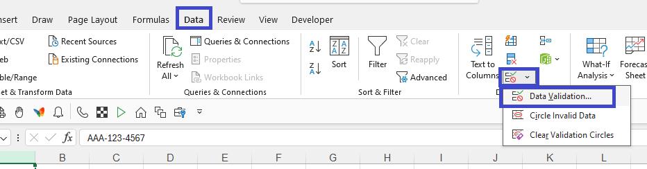
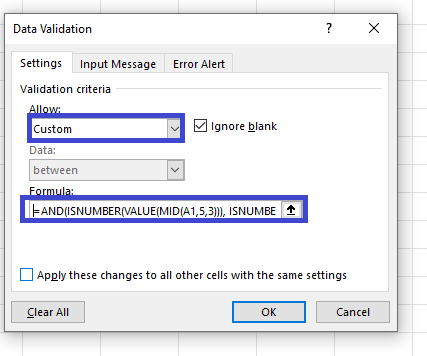
Select column A for example then from Data tab select Data Validation Select Custom and paste the formula This is the formula you can use =AND(ISNUMBER(VALUE(MID(A1,5,3))), ISNUMBER(VALUE(MID(A1,9,4))), ISERROR(VALUE(LEFT(A1,3))), MID(A1,4,1)="-", MID(A1,8,1)="-", LEN(A1)=12)
-
كود لإنشاء ملف نصي في مجلد النظام system
lionheart replied to فتحي محمد's topic in منتدى الاكسيل Excel
Try #If VBA7 Then Private Declare PtrSafe Function ShellExecute Lib "shell32.dll" Alias "ShellExecuteA" (ByVal hwnd As LongPtr, ByVal lpOperation As String, ByVal lpFile As String, ByVal lpParameters As String, ByVal lpDirectory As String, ByVal nShowCmd As Long) As LongPtr #Else Private Declare Function ShellExecute Lib "shell32.dll" Alias "ShellExecuteA" (ByVal hwnd As Long, ByVal lpOperation As String, ByVal lpFile As String, ByVal lpParameters As String, ByVal lpDirectory As String, ByVal nShowCmd As Long) As Long #End If Function CreateElevatedFile(ByVal sFilePath As String, ByVal sFileContent As String) As Boolean On Error GoTo ErrorHandler Dim fso As Object, sScriptPath As String, psScript As String, EscFilePath As String, EscContent As String sScriptPath = Environ("TEMP") & "\create_elevated_file.ps1" EscFilePath = Replace(Replace(sFilePath, "'", "''"), """", "\""") EscContent = Replace(Replace(sFileContent, "'", "''"), """", "\""") psScript = "$t = [System.Diagnostics.ProcessWindowStyle]::Hidden;$p = Start-Process -WindowStyle $t -FilePath 'powershell.exe' -ArgumentList '-Command ""Set-Content -Path \""" & EscFilePath & "\""` -Value \""" & EscContent & "\""""' -Verb RunAs -PassThru;$p.WaitForExit();Exit $p.ExitCode" Set fso = CreateObject("Scripting.FileSystemObject") With fso.CreateTextFile(sScriptPath, True) .WriteLine psScript .Close End With ShellExecute 0, "runas", "powershell.exe", "-ExecutionPolicy Bypass -WindowStyle Hidden -File """ & sScriptPath & """", vbNullString, 0 CreateElevatedFile = True Exit Function ErrorHandler: CreateElevatedFile = False End Function Sub Create_File_With_Elevated_Permissions() Dim success As Boolean success = CreateElevatedFile("C:\Windows\Test.txt", "This Was Created With Elevated Permissions") If success Then MsgBox "File Created Successfully", vbInformation Else MsgBox "File Not Created", vbExclamation End If End Sub -
تلوين السؤال بناء على الكلمة الاولي فى السؤال
lionheart replied to amr_ha2003's topic in منتدى الاكسيل Excel
Right-Click on sheet name and view code then paste the following Private Sub Worksheet_Change(ByVal Target As Range) If Target.Cells.CountLarge > 1 Then Exit Sub If Target.Column = 1 Then If Split(Target.Value, " ")(0) = "اكتب" Or Split(Target.Value, " ")(0) = "فكر" Then Target.Interior.Color = RGB(0, 112, 192) End If End If End Sub -
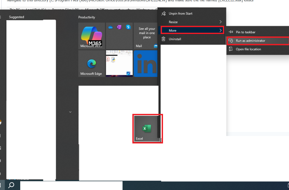
Navigate to this directory [C:\Program Files (x86)\Microsoft Office\root\vfs\Windows\SHELLNEW] and make sure the file named [EXCEL12.xlsx] exists If the file doesn't exist download it from the post (I will attach it for you) then copy it to the directory in the above screenshot Create an excel shortuct and right-click on it and select [Run as administrator] Finally execute the following code Sub Test() Const SEXCELFILE As String = "EXCEL12.xlsx" Dim subKeys, WshShell As Object, fso As Object, baseKeyPath As String, sFullKeyPath As String, sDestFile As String, sSourceFile As String, i As Integer Set WshShell = CreateObject("WScript.Shell") baseKeyPath = "HKEY_CURRENT_USER\Software\Classes\" subKeys = Array(".xlsx\", "Excel.Sheet.12\", "ShellNew\") sFullKeyPath = baseKeyPath For i = LBound(subKeys) To UBound(subKeys) sFullKeyPath = sFullKeyPath & subKeys(i) If Not RegKeyExists(WshShell, sFullKeyPath) Then WshShell.RegWrite sFullKeyPath, "" Next i sDestFile = "C:\Program Files (x86)\Microsoft Office\root\vfs\Windows\SHELLNEW\" & SEXCELFILE Set fso = CreateObject("Scripting.FileSystemObject") If Not fso.FileExists(sDestFile) Then sSourceFile = ThisWorkbook.Path & "\" & SEXCELFILE If fso.FileExists(sSourceFile) Then fso.CopyFile sSourceFile, sDestFile Else MsgBox "Source File '" & SEXCELFILE & "' Not Found.", vbExclamation: Exit Sub End If End If WshShell.RegWrite sFullKeyPath & "FileName", sDestFile, "REG_SZ" Set WshShell = Nothing: Set fso = Nothing MsgBox "Done", vbInformation End Sub Function RegKeyExists(WshShell As Object, regKey As String) As Boolean On Error Resume Next WshShell.RegRead regKey RegKeyExists = (Err.Number = 0) On Error GoTo 0 End Function EXCEL12.XLSX

-
Put your string in cell A1 then run the following code that will list all the characters and their count in column C and D Sub Count_All_Characters() Dim ch, arrKeys, arrValues, ws As Worksheet, dict As Object, txt As String, i As Long Set ws = ActiveSheet Set dict = CreateObject("Scripting.Dictionary") txt = ws.Range("A1").Value For i = 1 To Len(txt) ch = Mid(txt, i, 1) dict(ch) = dict(ch) + 1 Next i With ws .Columns("C:D").ClearContents .Range("C1:D1").Value = Array("Character", "Count") If dict.Count > 0 Then arrKeys = dict.Keys arrValues = dict.Items .Range("C2").Resize(dict.Count, 1).Value = Application.Transpose(arrKeys) .Range("D2").Resize(dict.Count, 1).Value = Application.Transpose(arrValues) End If End With Set dict = Nothing MsgBox "Done", 64 End Sub
-
Try this solution توزيع الدرجة.xlsm
-
You can use helper column as you can't directly use SUBTOTAL with COUNTIF but you can achieve that using SUMPRODUCT approach Suppose you have names in range B2:B6 and you want to count if the name starts with [Kh] letters Now you can try this formula =SUMPRODUCT(SUBTOTAL(103, OFFSET(B2:B6, ROW(B2:B6)-MIN(ROW(B2:B6)), 0, 1)) * EXACT(LEFT(B2:B6, 2), "Kh"))
-
Try this code Private Declare PtrSafe Function MakeSureDirectoryPathExists Lib "imagehlp.dll" (ByVal DirPath As String) As Boolean Sub Export_Range_As_Picture() Dim ws As Worksheet, oRng As Range, oChart As ChartObject, sFolder As String, sFile As String, rw As Long Application.ScreenUpdating = False Set ws = Sheet1 sFolder = "D:\Pic\" MakeSureDirectoryPathExists sFolder sFile = sFolder & ws.Range("A1").Value & "." & "jpg" rw = FindErrorRow(ws, 2) If rw <> -1 Then Set oRng = ws.Range("A2:E" & rw) Else Set oRng = ws.Range("A2:E" & ws.Cells(Rows.Count, "B").End(xlUp).Row) End If oRng.CopyPicture xlScreen, xlPicture Set oChart = ws.ChartObjects.Add(Left:=0, Top:=0, Width:=oRng.Width * 1, Height:=oRng.Height * 1) With oChart .Activate .Chart.Paste .Chart.Export Filename:=sFile .Delete End With Application.ScreenUpdating = True MsgBox "Done", 64 End Sub Function FindErrorRow(ByVal ws As Worksheet, ByVal col As Long) Dim rng As Range On Error Resume Next Set rng = ws.Columns(col).SpecialCells(xlCellTypeFormulas, xlErrors) On Error GoTo 0 If Not rng Is Nothing Then FindErrorRow = rng.Cells(1, 1).Row - 1 Else FindErrorRow = -1 End Function
-
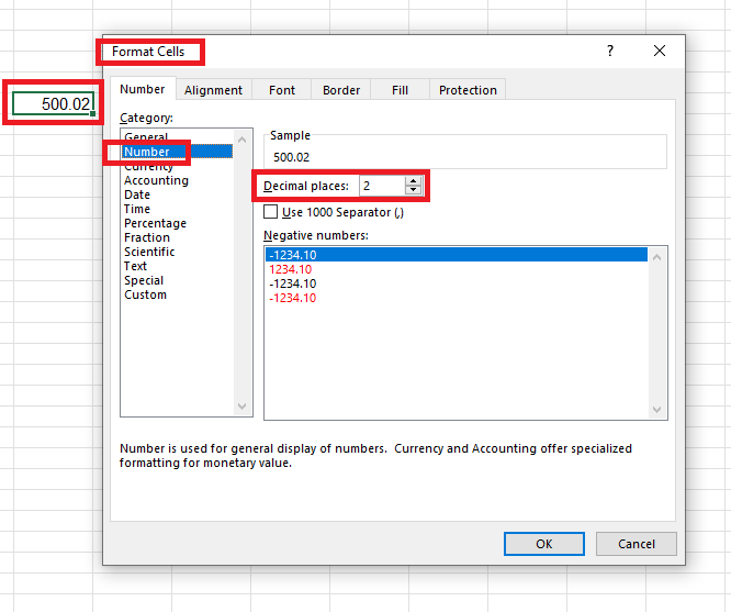
Right-Click on the cell >> Format Cells From Category select Number >> Change Decimal places to 2
-
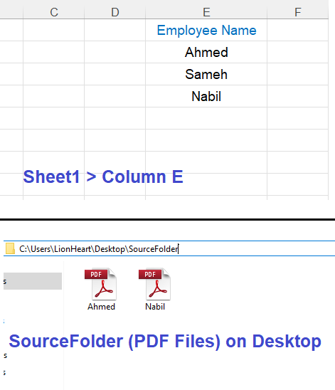
Hello Nabil Try this code Sub Move_PDF_Files() Dim ws As Worksheet, sDesktop As String, srcFolder As String, desFolder As String, empName As String, sFile As String, TargetFolder As String, lr As Long, r As Long Set ws = ThisWorkbook.Sheets("Sheet1") sDesktop = Environ("UserProfile") & "\Desktop\" srcFolder = sDesktop & "SourceFolder\" desFolder = sDesktop & "DestinationFolder\" If Dir(desFolder, vbDirectory) = "" Then MkDir desFolder lr = ws.Cells(Rows.Count, "E").End(xlUp).Row For r = 2 To lr empName = ws.Cells(r, "E").Value sFile = empName & ".pdf" TargetFolder = desFolder & empName & "\" If Dir(TargetFolder, vbDirectory) = "" Then MkDir TargetFolder If Dir(srcFolder & sFile) <> "" Then FileCopy srcFolder & sFile, TargetFolder & sFile Else Debug.Print "File [" & sFile & "] Not Found In Source Folder" End If Next r MsgBox "PDF Files Moved Successfully!", 64 End Sub This is for illustration
-
Try this instead Function MyRound(ByVal mainVal As Double, ByVal roundVal As Double) As Double Dim h As Double, v As Double On Error GoTo ErrSub h = roundVal / 2 If mainVal >= 0 Then If (mainVal Mod roundVal) >= h Then v = Application.WorksheetFunction.RoundUp(mainVal / roundVal, 0) * roundVal Else v = Application.WorksheetFunction.RoundDown(mainVal / roundVal, 0) * roundVal End If End If MyRound = v Exit Function ErrSub: MsgBox Err.Number & vbCrLf & Err.Description, vbCritical + vbMsgBoxRight MyRound = 0 End Function
-
احتاج دالة نقل بيانات من جدول بطريقة عمودية
lionheart replied to الشافعي's topic in منتدى الاكسيل Excel
Try this code Sub Test() Const SROW As Long = 6 Dim w, m As Long, r As Long, n As Long Application.ScreenUpdating = False With ActiveSheet .Columns("L:M").ClearContents m = SROW For r = SROW To .Cells(Rows.Count, "J").End(xlUp).Row n = .Cells(r, "I").Value If n > 0 Then .Cells(m, "L").Resize(n).Value = .Cells(r, "J").Value m = m + n End If Next r m = m - SROW w = Evaluate("ROW(1:" & m & ")") .Range("M" & SROW).Resize(UBound(w, 1)).Value = w End With Application.ScreenUpdating = True End Sub -
مساعدة فى تصدير بيانات من الليست بوكس الى ورقة العمل
lionheart replied to mody200's topic in منتدى الاكسيل Excel
The code is already OK as it exports data from the listbox to the worksheet Just comment out those two lines For X = 0 To ListBox1.ListCount - 1 Next X as I don't see any need to loop through the items of the listbox -
لدي ملف اكسيل و اريد نقل بيانات من شيت الي شيت اخر
lionheart replied to ahmedhassan1948's topic in منتدى الاكسيل Excel
In sheet [Template] put the formula in cell C3 =INDEX(Support!A:A,MATCH(Criteria,Support!B:B,0)) -
Try this formula =MID(LEFT(A1,LEN(A1)-6),5,LEN(LEFT(A1,LEN(A1)-6)))
-
Not so clear but try this code Sub Test() Dim a, letters, i As Long, ii As Long, k As Long a = Sheet1.Range("C1").CurrentRegion.Value Rem letters = Split("ا,أ,إ,آ", ",") letters = Split("ب", ",") ReDim b(1 To UBound(a, 1), 1 To UBound(a, 2)) For i = 2 To UBound(a, 1) If IsNumeric(Application.Match(Left(a(i, 2), 1), letters, 0)) Then k = k + 1 For ii = LBound(a, 2) To UBound(a, 2) b(k, ii) = a(i, ii) Next ii End If Next i If k > 0 Then With Sheet2 .Columns("C:E").ClearContents .Range("C1").Resize(, 3).Value = Sheet1.Range("C1").Resize(, 3).Value .Range("C2").Resize(k, UBound(b, 2)).Value = b End With End If End Sub
-
تحويل الاعداد من الحالة الافقية الى تسلسل راسي
lionheart replied to خير الايمان's topic in منتدى الاكسيل Excel
Try to read the code to add a fourth column in the output. The code is so simple to read -
تحويل الاعداد من الحالة الافقية الى تسلسل راسي
lionheart replied to خير الايمان's topic in منتدى الاكسيل Excel
Try Sub Test() Dim ws As Worksheet, m As Long, i As Long, ii As Long Application.ScreenUpdating = False Set ws = ActiveSheet: m = 2 With ws .Columns("K:M").Clear .Columns("M").ColumnWidth = 11 With .Range("K1").Resize(, 3) .Value = Array("Group", "Number", "Work Date") .Interior.Color = RGB(146, 205, 220) .HorizontalAlignment = xlCenter: .VerticalAlignment = xlCenter End With For i = 2 To 6 If .Cells(i, 2).Value < .Cells(i, 3).Value And IsNumeric(.Cells(i, 2).Value) And IsNumeric(.Cells(i, 2).Value) Then For ii = .Cells(i, 2).Value To .Cells(i, 3).Value .Cells(m, "K").Resize(, 3).Value = Array(.Cells(i, 1).Value, ii, .Cells(i, 4).Value) m = m + 1 Next ii End If Next i End With Application.ScreenUpdating = True End Sub -
تلوين خليه لو وجد مجلد اسمه بنفس قيمه الخليه
lionheart replied to تامر خليفه's topic in منتدى الاكسيل Excel
Do it yourself Press Alt + F11 >> Insert Module >> Paste the code -
تلوين خليه لو وجد مجلد اسمه بنفس قيمه الخليه
lionheart replied to تامر خليفه's topic in منتدى الاكسيل Excel
Try this code Sub Test() Dim ws As Worksheet, fso As Object, sPath As String, lr As Long, iRow As Long Set ws = ActiveSheet Set fso = CreateObject("Scripting.FileSystemObject") lr = ws.Cells(Rows.Count, 1).End(xlUp).Row ws.Columns(1).Interior.Color = xlNone For iRow = 2 To lr sPath = ThisWorkbook.Path & "\" & ws.Cells(iRow, 1).Value If fso.FolderExists(sPath) Then ws.Cells(iRow, 1).Interior.Color = vbGreen End If Next iRow End Sub -
Here's a version that merges cells although I see not practical and not useful later Sub Test() Dim ws As Worksheet, sh As Worksheet, lr As Long, r As Long, m As Long, n As Long, i As Long, c As Long Set ws = ThisWorkbook.Worksheets("1") Set sh = ThisWorkbook.Worksheets("2") lr = ws.Cells(Rows.Count, 1).End(xlUp).Row If lr < 6 Then Exit Sub m = 5: n = m Application.ScreenUpdating = False Application.DisplayAlerts = False With sh.Rows("5:" & Rows.Count) .ClearContents: .Borders.Value = 0: .UnMerge: .RowHeight = 20.25 End With For r = 6 To lr If ws.Cells(r, 4).Value > 0 Then For i = 1 To ws.Cells(r, 4).Value sh.Cells(m, 1).Value = ws.Cells(r, 2).Value sh.Cells(m, 2).Value = ws.Cells(r, 3).Value sh.Cells(m, 3).Value = ws.Cells(r, 4).Value sh.Cells(m, 4).Value = ws.Range("D3").Value & ws.Cells(r, 1).Value & ws.Cells(r, 2).Value & i m = m + 1 Next i For c = 1 To 3 With sh.Range(sh.Cells(n, c), sh.Cells(m - 1, c)) .Merge: .HorizontalAlignment = xlCenter: .VerticalAlignment = xlCenter End With Next c If lr = r Then Exit For sh.Cells(m, 1).Resize(, 4).Interior.Color = vbMagenta m = m + 1 n = m End If Next r sh.Range("A5:F" & m - 1).Borders.Value = 1 Application.DisplayAlerts = True Application.ScreenUpdating = True End Sub
-
Here's a modification to let empty row between results but I won't merge cells Sub Test() Dim ws As Worksheet, sh As Worksheet, lr As Long, r As Long, m As Long, i As Long Set ws = ThisWorkbook.Worksheets("1") Set sh = ThisWorkbook.Worksheets("2") lr = ws.Cells(Rows.Count, 1).End(xlUp).Row If lr < 6 Then Exit Sub m = 5 Application.ScreenUpdating = False For r = 6 To lr If ws.Cells(r, 4).Value > 0 Then For i = 1 To ws.Cells(r, 4).Value sh.Cells(m, 1).Value = ws.Cells(r, 2).Value sh.Cells(m, 2).Value = ws.Cells(r, 3).Value sh.Cells(m, 3).Value = ws.Cells(r, 4).Value sh.Cells(m, 4).Value = ws.Range("D3").Value & ws.Cells(r, 1).Value & ws.Cells(r, 2).Value & i m = m + 1 Next i If lr = r Then Exit For sh.Cells(m, 1).Resize(, 4).Interior.Color = vbMagenta m = m + 1 End If Next r Application.ScreenUpdating = True End Sub
-
Delete the rows in sheet2 from row 5 to row 25 then try this code Sub Test() Dim ws As Worksheet, sh As Worksheet, lr As Long, r As Long, m As Long, i As Long Set ws = ThisWorkbook.Worksheets("1") Set sh = ThisWorkbook.Worksheets("2") lr = ws.Cells(Rows.Count, 1).End(xlUp).Row If lr < 6 Then Exit Sub m = 5 Application.ScreenUpdating = False For r = 6 To lr If ws.Cells(r, 4).Value > 0 Then For i = 1 To ws.Cells(r, 4).Value sh.Cells(m, 1).Value = ws.Cells(r, 2).Value sh.Cells(m, 2).Value = ws.Cells(r, 3).Value sh.Cells(m, 3).Value = ws.Cells(r, 4).Value sh.Cells(m, 4).Value = ws.Range("D3").Value & ws.Cells(r, 1).Value & ws.Cells(r, 2).Value & i m = m + 1 Next i End If Next r Application.ScreenUpdating = True End Sub I didn't merge the cells as it is not practical
-
Whar are the expected correct results exactly I have tried UDF on my side and these are the results 04-11-04 04-11-00 04-10-30 04-10-29 04-10-28 04-10-27 04-10-26