lionheart

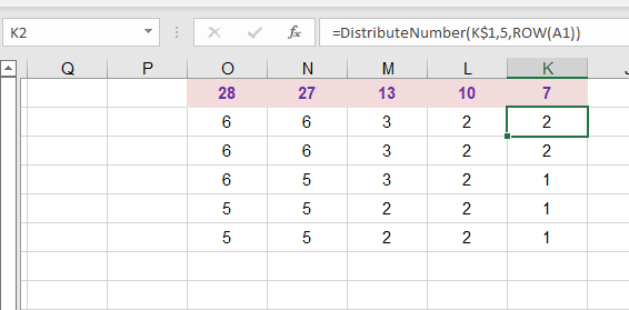
Here's a modified udf to be compatible with older versions of excel Function DistributeNumber(ByVal num As Long, ByVal chunks As Long, ByVal iIndex As Long) Dim i As Long ReDim b(chunks - 1) For i = 0 To chunks - 1 If i = chunks - 1 Then b(i) = num Else b(i) = WorksheetFunction.RoundUp(num / (chunks - i), 0) num = num - b(i) End If Next i On Error Resume Next DistributeNumber = b(iIndex - 1) If Err.Number <> 0 Then DistributeNumber = vbNullString: Err.Clear On Error GoTo 0 End Function you can use the udf as formula (but you will have to drag the formula) Say the number is K1 so the formula in cell K2 should be =DistributeNumber(K$1,5,ROW(A1)) Drag the formula down to get the results

It works well at my side Have a look May be the problem is that I have a new version of excel (office 365) paste the code and press Ctrl + G to see the results in the immediate window Sub Test() Dim a, e For Each e In Array(7, 10, 13) a = DistributeNumber(Val(e), 5) Debug.Print Join(a, "-") Next e End Sub Function DistributeNumber(ByVal num As Long, ByVal chunks As Long) Dim i As Long ReDim b(chunks - 1) For i = 0 To chunks - 1 If i = chunks - 1 Then b(i) = num Else b(i) = WorksheetFunction.RoundUp(num / (chunks - i), 0) num = num - b(i) End If Next i DistributeNumber = b End Function

Not sure what is the problem now Try the solution first and tell me if there is a problem in distribution and use images please

Try this udf Function DistributeNumber(ByVal num As Long, ByVal chunks As Long) Dim i As Long ReDim b(chunks - 1) For i = 0 To chunks - 1 If i = chunks - 1 Then b(i) = num Else b(i) = WorksheetFunction.RoundUp(num / (chunks - i), 0) num = num - b(i) End If Next i DistributeNumber = b End Function The udf can be used as formula =TRANSPOSE(DistributeNumber(13,5))

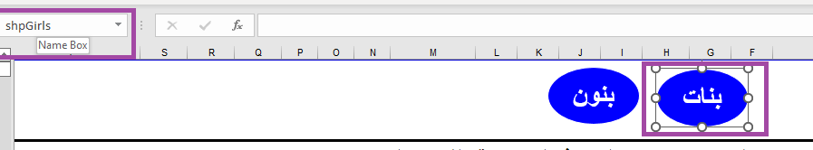
Rename the shapes from NAME BOX not the text on the shape Assign the same macro for both the shapes. I have tried at my side and the code works well Another point, you haven't execute the macro directly from the visual basic editor It has to be assigned to a shape

I have no time to create a file to test on it Please attach sample file if you really need help

The file is not perfect file as it has a lot of formulas that make the file slow. Generally follow the steps accurately to solve the problem of sort First select the shape that has the caption GIRLS and rename the shape from the Name Box to shpGirls Do the same step with the shape of BOYS and rename it to shpBoys Insert new module and paste the code Sub Sort_By_Boys_Girls() Dim shp As Shape, lr As Long, n As Long Application.ScreenUpdating = False Application.Calculation = xlCalculationManual Set shp = ActiveSheet.Shapes(Application.Caller) If shp.Name = "shpGirls" Then n = 1 Else n = 2 With ActiveSheet lr = .Cells(Rows.Count, "D").End(xlUp).Row With .Sort .SortFields.Clear .SortFields.Add Key:=Range("F9"), Order:=xlAscending .SortFields.Add Key:=Range("I9"), Order:=n .SortFields.Add Key:=Range("D9"), Order:=xlAscending .SetRange ActiveSheet.Range("D9:AH" & lr) .Header = xlNo .Apply End With End With Application.Calculation = xlCalculationAutomatic Application.ScreenUpdating = True End Sub Finally assign the macro named [Sort_By_Boys_Girls] to both the shapes

Don't post mysterious questions. Be specific and attach file with the desired results

Attach the file that has the problem. More details will help others to offer help

The topic must be CLOSED as you did not respond properly to Mohamed Hicham in a good way Generally, I will share my idea but I will not extend my reply if you have more questions First create a userform with TextBox1 & ListBox1 controls Second paste the following code on userform module Option Explicit Private arrData, ws As Worksheet Private Sub UserForm_Initialize() Dim lr As Long Set ws = ThisWorkbook.Worksheets(1) lr = ws.Cells(ws.Rows.Count, "C").End(xlUp).Row arrData = ws.Range("C3:C" & lr).Value Me.ListBox1.List = Application.Transpose(arrData) End Sub Private Sub TextBox1_Change() Dim txt As String, i As Long Me.ListBox1.Clear If Len(Me.TextBox1.Value) = 0 Then Me.ListBox1.List = Application.Transpose(arrData): Exit Sub txt = Me.TextBox1.Value For i = LBound(arrData) To UBound(arrData) If InStr(LCase(arrData(i, 1)), LCase(txt)) > 0 Then Me.ListBox1.AddItem arrData(i, 1) End If Next i End Sub Private Sub ListBox1_DblClick(ByVal Cancel As MSForms.ReturnBoolean) Dim x x = Application.Match(ListBox1.Value, ws.Columns(3), 0) With ws.Range("H3").Resize(, 4) .ClearContents If Not IsError(x) Then .Value = ws.Range("B" & x).Resize(, 4).Value Unload Me End If End With End Sub Now right-click the worksheet name and select [View Code] and paste the following code Option Explicit Private Sub Worksheet_BeforeDoubleClick(ByVal Target As Range, Cancel As Boolean) If Target.Address = "$H$3" Then Cancel = True UserForm1.Show End If End Sub The code usage -------------------- Double click on cell H3 and the form will be shown then type some letters of the name you need to search and finally double click the name on the listbox to get the results in the range H3 to K3 Regards

More details about the error may help Please post a picture of the error message that appears to you Is that the original file without any changes or you have changed it

Try this formula =IF(C5="","",IF(AND(C5>$A$2,C5<=$B$2)=FALSE,"Not Calculated",IF(COUNTIF($A$5:$A5,A5)>3,"Not Rounded","Calculated")))

The code works on both tables on my side

Try this modification Option Explicit Sub Draw_Circles() Const nMax As Integer = 30 Dim mx, ws As Worksheet, v As Shape, x As Integer, r As Long, c As Long, cnt As Long Call Remove_Circles x = ActiveWindow.Zoom Application.ScreenUpdating = False Set ws = ThisWorkbook.Worksheets("ty") ActiveWindow.Zoom = 100 mx = ws.Range("N2").Value If mx = 0 Or Not IsNumeric(mx) Then MsgBox "Enter Valid Number In Cell N2", vbExclamation: GoTo Skipper For c = 10 To 8 Step -1 For r = 4 To 14 Step 2 With ws.Cells(r, c) If .Value <> "" Then cnt = cnt + 1 Set v = .Parent.Shapes.AddShape(msoShapeOval, .Left + 1, .Top + 1, .Width - 2, .Height - 2) v.Fill.Visible = msoFalse v.Line.ForeColor.SchemeColor = 10 v.Line.Weight = 1 If cnt = mx Then Exit For End If End With Next r If cnt = mx Then Exit For Next c cnt = 0 For c = 2 To 10 For r = 20 To 30 Step 2 With ws.Cells(r, c) If .Value <> "" Then cnt = cnt + 1 Set v = .Parent.Shapes.AddShape(msoShapeOval, .Left + 1, .Top + 1, .Width - 2, .Height - 2) v.Fill.Visible = msoFalse v.Line.ForeColor.SchemeColor = 10 v.Line.Weight = 1 If cnt = nMax Then Exit For End If End With Next r If cnt = nMax Then Exit For Next c Skipper: ActiveWindow.Zoom = x Application.ScreenUpdating = True MsgBox "Done...", 64 End Sub Sub Remove_Circles() Dim shp As Shape For Each shp In ActiveSheet.Shapes If shp.AutoShapeType = msoShapeOval Then shp.Delete Next shp End Sub

Another one using office 365 =LET(x,MID(A1,SEQUENCE(LEN(A1)),1),FILTER(x,SUBSTITUTE(x," ","")<>""))

Very bad approach to use macro recorder Generally try the code that do the same steps Sub Test() Dim rng As Range, lr As Long With ActiveSheet If .Range("A10").Value = Empty Then MsgBox "Enter Number", vbExclamation: Exit Sub Application.ScreenUpdating = False Set rng = .Range("A10").Resize(, 9) lr = .Cells(Rows.Count, "Z").End(xlUp).Row + 1 .Range("Z" & lr).Resize(, 9).Value = rng.Value rng.SpecialCells(xlCellTypeConstants).ClearContents Application.ScreenUpdating = True End With End Sub

Don't forget to remove all the codes in your file before executing the code I posted

Hello. Try the following code that is not exactly as you need but give it a try All the bills will be exported to only one pdf to Desktop instead of creating a pdf for each bill Sub Export_All_Bills_To_One_PDF() Dim bill, wb As Workbook, wsData As Worksheet, wsBill As Worksheet, wsCounter As Worksheet, shp As Shape, lr As Long, ls As Long, r As Long, m As Long, n As Long Application.ScreenUpdating = False With ThisWorkbook Set wsData = .Worksheets(1): Set wsBill = .Worksheets(2): Set wsCounter = .Worksheets(3) End With lr = wsCounter.Cells(Rows.Count, "A").End(xlUp).Row ls = wsData.Cells(Rows.Count, "B").End(xlUp).Row Set wb = Workbooks.Add(xlWBATWorksheet) For r = 2 To lr wsBill.Range("D1").Value = wsCounter.Cells(r, 1).Value bill = wsBill.Range("A2").Value wsBill.Range("A6:B30").ClearContents: n = 6 For m = 3 To ls If wsData.Cells(m, "B").Value = bill Then wsBill.Range("A" & n).Resize(, 2).Value = wsData.Range("C" & m).Resize(, 2).Value n = n + 1 End If Next m wsBill.Copy After:=wb.Worksheets(wb.Worksheets.Count) With ActiveSheet .Range("A2").Value = .Range("A2").Value .Range("D1").ClearContents For Each shp In .Shapes shp.Delete Next shp End With Next r Application.DisplayAlerts = False wb.Worksheets(1).Delete Application.DisplayAlerts = True wb.ExportAsFixedFormat Type:=xlTypePDF, Filename:=Environ("USERPROFILE") & "\Desktop\" & "All_Bills.pdf", OpenAfterPublish:=True wb.Close SaveChanges:=False Application.ScreenUpdating = True End Sub

The topic is just for one problem and I think this is solved If you need more help, please post a new topic with only one request in the new topic The forum is not for making all the work for you

I don't know what do you want exactly. Focus on just one problem

I am confused. What's the problem exactly Try to be specific

Try Sub Test() Dim ws As Worksheet, sh As Worksheet, tbl As ListObject, lr As Long, i As Long Application.ScreenUpdating = False With ThisWorkbook Set ws = .Worksheets("Items"): Set sh = .Worksheets("Orders") End With Set tbl = sh.ListObjects(1) lr = tbl.Range.Rows.Count + tbl.Range.Row - 1 Do While sh.Cells(lr, "C").Value = Empty lr = lr - 1 Loop lr = lr + 1 Dim a(1 To 16), e For Each e In Split("H15,F4,F6,H6,F9,H9,J9,F13,H13,J13,F15,J15,F18,H18,J18,F20", ",") i = i + 1 a(i) = ws.Range(e).Value Next e sh.Range("C" & lr).Resize(, 16).Value = a Application.ScreenUpdating = True MsgBox "Done", 64 End Sub

Very weird I have commented this line as I didn't want to print Rem sh.PrintOut Rem is used to make the line as a comment. Just remove the Rem and the sheet will be printed Another point I have put this line just for wait, you can remove this line Application.Wait Now + TimeValue("00:00:01") Try to understand the code. Don't wait others to do the whole work for you

Try Sub Test() Dim a, e, ws As Worksheet, sh As Worksheet, i As Long Set ws = ThisWorkbook.Worksheets(1): Set sh = ThisWorkbook.Worksheets(2) a = ws.Range("B11:J" & ws.Cells(Rows.Count, "B").End(xlUp).Row).Value e = sh.Range("Q3").Value For i = LBound(a) To UBound(a) If a(i, 8) = e Then sh.Range("F9").Value = a(i, 2) sh.Range("M9").Value = a(i, 9) Application.Wait Now + TimeValue("00:00:01") Rem sh.PrintOut End If Next i End Sub

Try Sub Test() Dim lr As Long With ActiveSheet lr = .Cells(Rows.Count, 1).End(xlUp).Row With .Sort .SortFields.Clear .SortFields.Add Key:=Range("F3"), Order:=xlAscending .SortFields.Add Key:=Range("G3"), Order:=xlDescending .SortFields.Add Key:=Range("H3"), Order:=xlAscending .SetRange ActiveSheet.Range("A3:H" & lr) .Header = xlYes .Apply End With End With End Sub